Author: Zach Christoff
Lab Partner: Daniel Baka
Date: 9/30/15
Lab Partner: Daniel Baka
Date: 9/30/15
Purpose
I will investigate the position, velocity and acceleration associated with motion.
Theory
For this lab, we will use kinematic equations to determine the position, velocity and acceleration at a given second. Below are the basic shapes of the graphs along with the kinematic equations that create their shapes.

|

|

|

|

|

|
Experimental Technique
To measure the motion of a cart, a ticker timer was attached to a decline place. A piece of paper was strung through the ticker timer and attached to the back of the cart. As the cart moves down the plane, a carbon mark is made on the paper every 1/40th of a second.

|

|
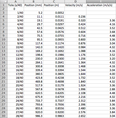
Data


Analysis
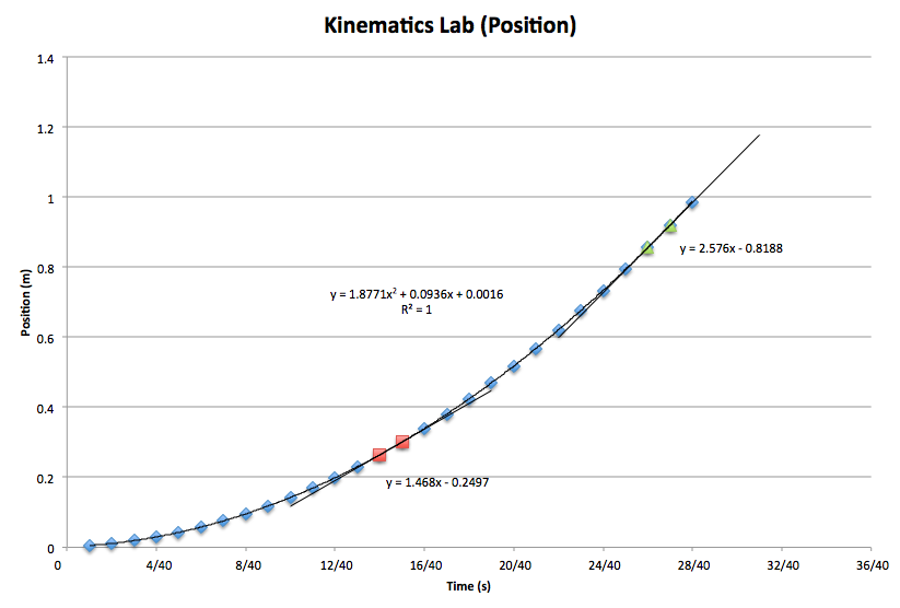
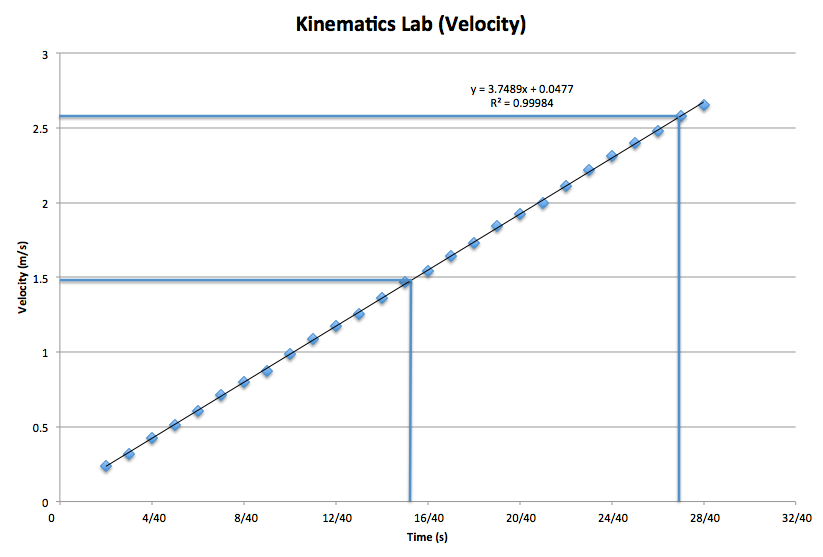
According to both the position and velocity graphs in the data, the velocity of the cart at the 75cm and 15cm mark can be determined. For the position, the slope of the secant line determines the velocity.


|
At 75cm, the slope of the secant line is 1.468. This means the velocity is 1.468 m/s. Likewise, the slope of the secant line at 15cm is 2.576, which means the velocity is 2.567 m/s.
The velocity can also be determined by simply looking at the velocity graph. If lines are drawn up and over at the 75cm and 15cm mark, the velocity coincides with the slope of the secant line.
Excel was used to easily calculate velocity and acceleration. However, formulas needed to be input in order for Excel to follow through with the calculations.
Cell D4: Velocity = (change in position)/t Velocity = (C4 - C3)/t Velocity = (0.0111 - 0.0052)40 Velocity = 0.236 Cell E5 Acceleration = (change in velocity)/t Acceleration = (D5 - D4)/t Acceleration = (0.320 - 0.236)40 Acceleration = 3.36 |
Conclusion
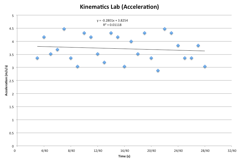
The graphs shown above represent the motion of the cart down an incline plane. According to my data, acceleration does not appear constant. However, acceleration is constant, but there is some error associated with measurements and calculations.
In the Data section, the position graph uses the kinematic equation that takes the form of a parabolic equation, as stated below the graph. The same applies for the velocity graph; a kinematic equation that represents a line is shown below the graph. Acceleration is constant, so therefore there is a horizontal line at a designated "y" value, which represents acceleration.
The only possible sources of friction in this lab are the wheels on the cart and paper from the ticker timer. However, these sources contain very minimal sources of friction and should not throw the numbers off very much, or even at all.
The "noisiness" in the acceleration graph is due to the uncertainty made in the measurements. There is parallax error in measuring the dots, which I tried to eliminate by looking directly above them at eye level. Since acceleration is constant, velocity should be increasing at a constant rate. Since the numbers in my data table aren't exact, acceleration cannot be exact either since it is based off of the velocity numbers.
References
Giancoli, Douglas C. Physics: Principles with Applications. 5th ed. Upper Saddle River, N.J.: Prentice Hall, 1998. Print.
